About

These blogs are my notes that represent my interpretation of the CS236 course taught by Stefano.

Recap

• Autoregressive models:
  • Chain rule based factorization is fully general
  • Compact representation via conditional independence and/or neural parameterizations
• Autoregressive models

  • Pros:

    • Easy to evaluate likelihoods
    • Easy to train

  • Cons:

    • Requires an ordering
    • Generation is sequential
    • Cannot learn features in an unsupervised way

Latent Variable Models: Introduction

• Lots of variability in images x due to gender, eye color, hair color, pose, etc. However, unless images are annotated, these factors of variation are not explicitly available (latent).

• Idea: explicitly model these factors using latent variables z

Latent Variable Models: Motivation

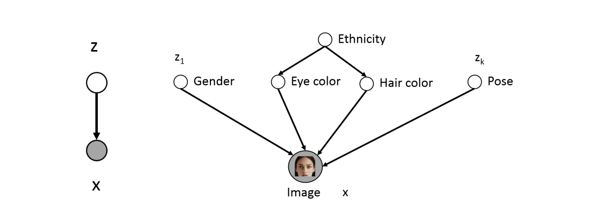
• Only shaded variables x are observed in the data (pixel values)
• Latent variables z correspond to high level features
  • If z chosen properly, p(x|z) could be much simpler than p(x)
  • If we had trained this model, then we could identify features via p(z | x), e.g., p(EyeColor = Blue|x)

Challenge: Very difficult to specify these conditionals by hand

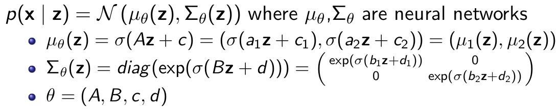
Deep Latent Variable Models

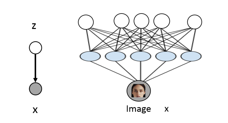
• Use neural networks to model the conditionals (deep latent variable models):
  • z ∼ N (0, I )
  • p(x | z) = N (µθ (z), Σθ (z)) where µθ ,Σθ are neural networks
• Hope that after training, z will correspond to meaningful latent factors of variation (features). Unsupervised representation learning.
• As before, features can be computed via p(z | x)

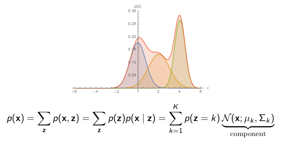
Mixture of Gaussians: a Shallow Latent Variable Model

• z ∼ Categorical(1, · · · , K )
• p(x | z = k) = N (µk , Σk )

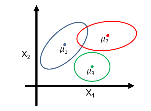
Generative process

• Pick a mixture component k by sampling z
• Generate a data point by sampling from that Gaussian

By learning p(x|z) we can do clustering by using p(z|x) as shown in the above image.

Another advantage is that Gaussian distribution is a simple one. And might not model p(x|z) properly but by mixing multiple Gaussian models for each conditional we get a complex distribution that can approximate the true data distribution

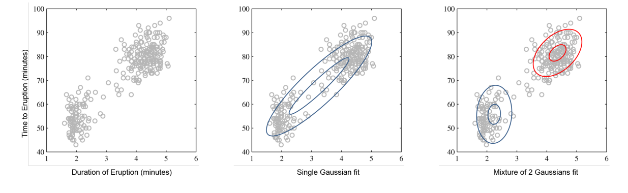
Variational Autoencoder

Extending the concept of mixture of gaussians discussed in last section, a variational autoencoder can be thought of as a mixture of gaussians of infinite Gaussians

• z ∼ N (0, I )
• 
• Even though p(x | z) is simple, the marginal p(x) is very complex/flexible

Marginal Likelihood

• Suppose some pixel values are missing at train time (e.g., top half)
• Let X denote observed random variables, and Z the unobserved ones (also called hidden or latent)
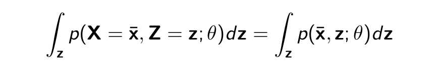
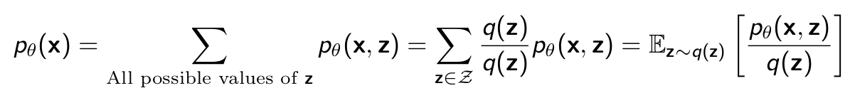
• Suppose we have a model for the joint distribution (e.g., PixelCNN) = p(X, Z; θ) What is the probability p(X = x̄; θ) of observing a training data point x̄?
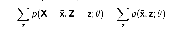
• Need to consider all possible ways to complete the image (fill green part)

Marginal Likelihood (Autoencoder)

A mixture of an infinite number of Gaussians:

• z ∼ N (0, I )
• p(x | z) = N (µθ (z), Σθ (z)) where µθ ,Σθ are neural networks
• Z are unobserved at train time (also called hidden or latent)
• Suppose we have a model for the joint distribution. What is the probability p(X = x̄; θ) of observing a training data point x̄?

Marginal Likelihood Continued..

• Considering the same joint distribution used to describe unobserved variables i.e p(X, Z; θ)
• We have a dataset D, where for each datapoint the X variables are observed (e.g., pixel values) and the variables Z are never observed (e.g., cluster or class id.) D = {x(1) , · · · , x(M) }.
• Maximum likelihood learning:

• 
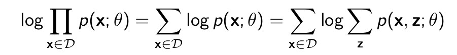
• Need approximations. One gradient evaluation per training data point x ∈ D, so approximation needs to be cheap.

Using Monte Carlo

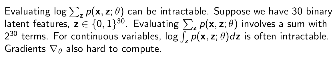
Likelihood function pθ (x) for Partially Observed Data is hard to compute:

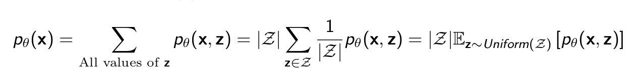
We can think of it as an (intractable) expectation. Monte Carlo to the rescue:

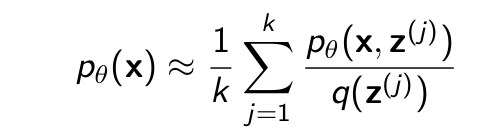
• Sample z(1) , · · · , z(k) uniformly at random
• Approximate expectation with sample average

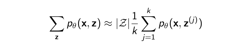
Works in theory but not in practice. For most z, pθ (x, z) is very low (most completions don’t make sense). Some completions have large pθ (x, z) but we will never ”hit” likely completions by uniform random sampling. Need a clever way to select z(j) to reduce variance of the estimator.

What do we do? Could try to learn a way to sample z that is more likely to help us observe p(x)..

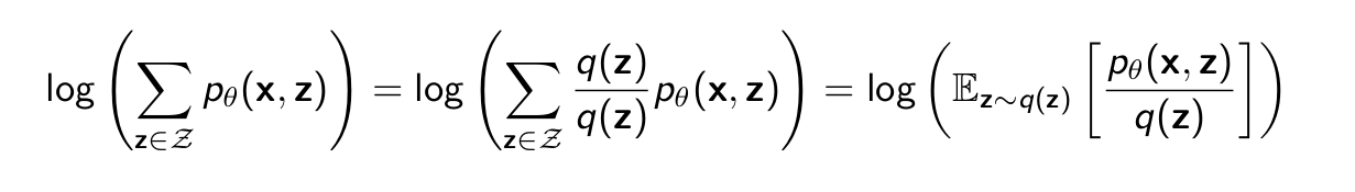
Importance Sampling

Instead of using a z/z solution we introduce q(z) where q(z) is a probablity distribution from which we sample z that are more likely to complete x.

Monte Carlo to the rescue:

• Sample z(1) , · · · , z(k) from q(z)
• Approximate expectation with sample average

Calculating log likelihood

Likelihood function pθ (x) for Partially Observed Data is hard to compute:

Monte Carlo to the rescue:

• Sample z(1) , · · · , z(k) from q(z)
• Approximate expectation with sample average

For training, we need the log-likelihood log (pθ (x)). We could estimate it as:

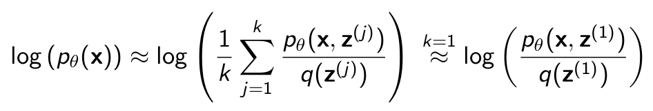
And for the same case of k=1 if we calculate the log of expectation without the monte carlo approximation. We see a potential problem

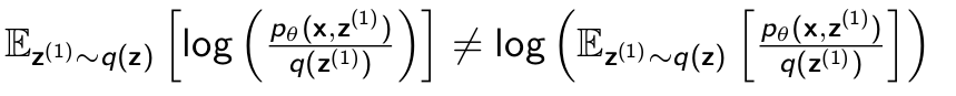
On the right hand side is the log of the expectation of sampling a single z from q(z) and on the left hand side is the output of the monte carlo approximation. It is clear that both of the values are not the same thing for k=1. For a higher k it might be same but for the base case we see that our estimation is not good.

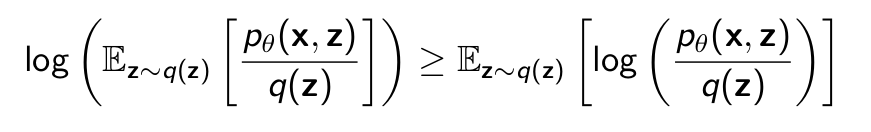
Evidence Lower Bound

The Log-Likehlihood for partially missing data is hard to compute.

log() is a concave function. log(px + (1 − p)x′) ≥ p log(x) + (1 − p) log(x′).

Using Jensen Equality we approximate the Log Likelihood as given. It is called ELBO or Evidence Lower Bound where our goal is to maximize the ELBO as much as possible

Variational Inference

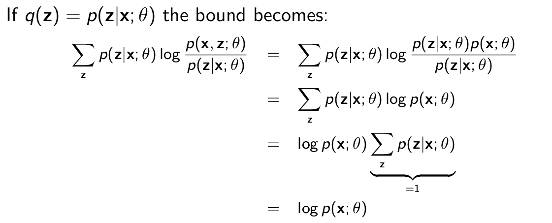
ELBO is maximum or equal when q = p(z|x; θ)

Proof:

• Confirms our previous importance sampling intuition: we should choose likely completions.

KL-Divergence relation with ELBO

Suppose q(z) is any probability distribution over the hidden variables. A little bit of algebra reveals

Corresponding proof. External link

Equality holds if q = p(z|x; θ) because DKL (q(z)∥p(z|x; θ))=0

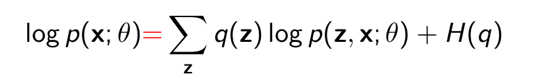
Then we can rewrite as follows.

Which means -> Minimizing KL-Divergence is equal to maximimzing ELBO

Computing q

• What if the posterior p(z|x; θ) is intractable to compute?
• Suppose q(z; ϕ) is a (tractable) probability distribution over the hidden variables parameterized by ϕ (variational parameters)
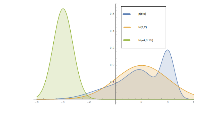
  • For example, a Gaussian with mean and covariance specified by ϕ q(z; ϕ) = N (ϕ1 , ϕ2 )
• Variational inference: pick ϕ so that q(z; ϕ) is as close as possible to p(z|x; θ). In the figure, the posterior p(z|x; θ) (blue) is better approximated by N (2, 2) (orange) than N (−4, 0.75) (green)

Variational approximation of the posterior

• Assume p(xtop , xbottom ; θ) assigns high probability to images that look like digits. In this example, we assume z = xtop are unobserved (latent)

• Suppose q(xtop ; ϕ) is a (tractable) probability distribution over the hidden variables (missing pixels in this example) xtop parameterized by ϕ (variational parameters)

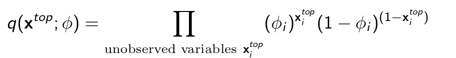
• Is ϕi = 0.5 ∀i a good approximation to the posterior p(xtop |xbottom ; θ)? No
• Is ϕi = 1 ∀i a good approximation to the posterior p(xtop |xbottom ; θ)? No
• Is ϕi ≈ 1 for pixels i corresponding to the top part of digit 9 a good approximation? Yes

Closing notes

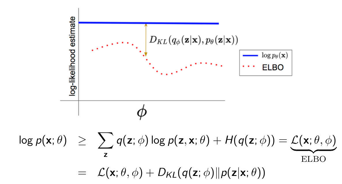
The better q(z; ϕ) can approximate the posterior p(z|x; θ), the smaller DKL (q(z; ϕ)∥p(z|x; θ)) we can achieve, the closer ELBO will be to log p(x; θ). Next: jointly optimize over θ and ϕ to maximize the ELBO over a dataset

• Latent Variable Models Pros:

  • Easy to build flexible models
  • Suitable for unsupervised learning

• Latent Variable Models Cons:

  • Hard to evaluate likelihoods
  • Hard to train via maximum-likelihood
  • Fundamentally, the challenge is that posterior inference p(z | x) is hard. Typically requires variational approximations

• Alternative: give up on KL-divergence and likelihood (GANs)