About

These blogs are my notes that represent my interpretation of the CS236 course taught by Stefano.

Recap

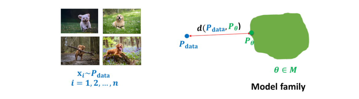
Learning a generative model.

• We are given a training set of examples, e.g., images of dogs

• We want to learn a probability distribution p(x) over images x such that

  • Generation: If we sample xnew ∼ p(x), xnew should look like a dog (sampling)
  • Density estimation: p(x) should be high if x looks like a dog, and low otherwise (anomaly detection)
  • Unsupervised representation learning: We should be able to learn what these images have in common, e.g., ears, tail, etc. (features)

• First question: how to represent pθ(x). Second question: how to learn it.

Defining the setting

• Lets assume that the domain is governed by some underlying distribution Pdata
• We are given a dataset D of m samples from Pdata
  • Each sample is an assignment of values to (a subset of) the variables, e.g., (Xbank = 1, Xdollar = 0, …, Y = 1) or pixel intensities.
• The standard assumption is that the data instances are independent and identically distributed (IID)
• We are also given a family of models M, and our task is to learn some “good” distribution in this set:
  • For example, M could be all Bayes nets with a given graph structure, for all possible choices of the CPD tables
  • For example, a FVSBN for all possible choices of the logistic regression parameters , θ = concatenation of all logistic regression coefficients

We have defined a way already in the last blog to represent probablity distributions in terms of parameters. But how do we find a model that captures the real data distribution as closely as possible. What are the factors to keep in mind?

That depends on the type of task.

• For Density estimation: we are interested in the full distribution (so later we can compute whatever conditional probabilities we want)

• Specific prediction tasks: we are using the distribution to make a prediction. Is this email spam or not? Structured prediction: Predict next frame in a video, or caption given an image. In these cases we might not have to compute full distribution if we assume that the input given for prediction is valid. So we are more interested in correctly modelling the conditional probablity.

• Structure or knowledge discovery: we are interested in the model itself. Usecases related to xAI

  • How do some genes interact with each other?
  • What causes cancer?

Learning as density estimation

• We want to learn the full distribution so that later we can answer any probabilistic inference query
• In this setting we can view the learning problem as density estimation
• We want to construct Pθ as ”close” as possible to Pdata (recall we assume we are given a dataset D of samples from Pdata )

But how do we evaluate closeness?

KL-divergence

• How should we measure distance between distributions?

• The Kullback-Leibler divergence (KL-divergence) between two distributions p and q is defined as

• D(p ∥ q) ≥ 0 for all p, q, with equality if and only if p = q.

Intuition behind KL Divergence

Assume that we have samples from the true data distribution Pdata and we learned a model Pθ parameterized by θ then KL Divergence can be thought of as the extra bits required to represent samples from Pdata by using the learned distribution Pθ instead. Normally using less bits would mean that Pθ is very close to Pdata.

Maximum Log Likelihood

Simplifying the KL Divergence as follows

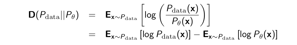
• The first term does not depend on Pθ .
• Then, minimizing KL divergence is equivalent to maximizing the expected log-likelihood
• Asks that Pθ assign high probability to instances sampled from Pdata , so as to reflect the true distribution
• Because of log, samples x where Pθ (x) ≈ 0 weigh heavily in objective
• Although we can now compare models, since we are ignoring H(Pdata ) = −Ex∼Pdata [log Pdata (x)], we don’t know how close we are to the optimum
• Problem: In general we do not know Pdata .

Maximum Likelihood

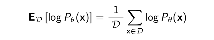
• Approximate the expected log-likelihood
  Ex∼Pdata [log Pθ (x)]
  with the empirical log-likelihood:

• Maximum likelihood learning is then:

• Equivalently, maximize likelihood of the data

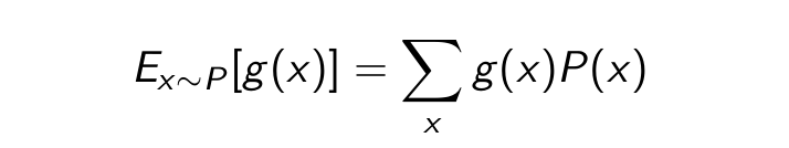
Monte Carlo Estimation

• Express the quantity of interest as the expected value of a random variable.

• Generate T samples x1 , . . . , xT from the distribution P with respect to which the expectation was taken.

• Estimate the expected value from the samples using

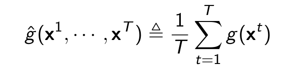
where x1 , . . . , xT are independent samples from P.

Intuition?

Most cases P(x) or the true data distribution might not be known. In that case sampling from the dataset and approximating the expected value according to Monte-Carle Estimation gives us a way to calculate the quantity of interest. In later sections the Monte Carlo Estimation will be used in derivations which would depict the usefulness of this approximation.

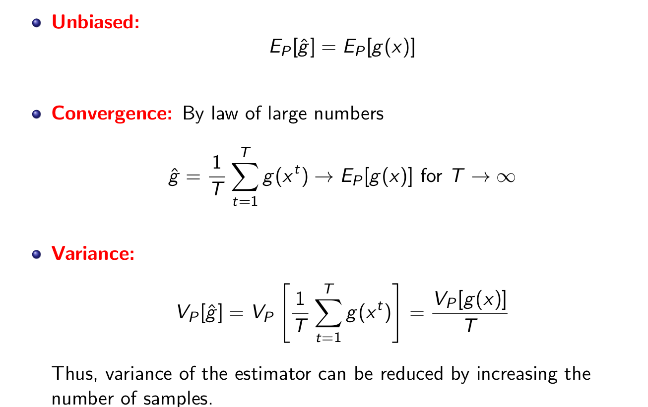
Properties of Monte Carlo Estimation

Estimating Pθ (x) via MLE

Example

• Single variable example: A biased coin
• Two outcomes: heads (H) and tails (T )
• Data set: Tosses of the biased coin, e.g., D = {H, H, T , H, T }
• Assumption: the process is controlled by a probability distribution Pdata (x) where x ∈ {H, T }
• Class of models M: all probability distributions over x ∈ {H, T }.
• Example learning task: How should we choose Pθ (x) from M if 3 out of 5 tosses are heads in D?

MLE scoring for the coin example

• We represent our model: Pθ (x = H) = θ and Pθ (x = T ) = 1 − θ
• Example data: D = {H, H, T , H, T }
• Likelihood of data: mult(Pθ (xi )) for i = θ · θ · (1 − θ) · θ · (1 − θ)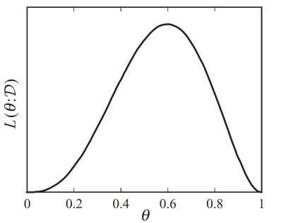
• Optimize for θ which makes D most likely. What is the solution in this case? θ = 0.6, optimization problem can be solved in closed-form

Extending the MLE principle to autoregressive models

Given an autoregressive model with n variables and factorization

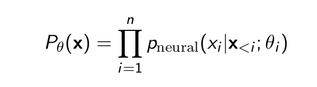
θ = (θ1 , · · · , θn ) are the parameters of all the conditionals. Training data
D = {x(1) , · · · , x(m) }. Maximum likelihood estimate of the parameters θ?

• Decomposition of Likelihood function

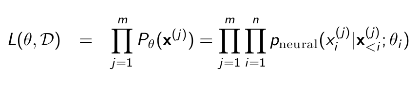
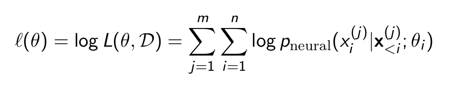
• Goal : maximize arg maxθ L(θ, D) = arg maxθ log L(θ, D)
• We no longer have a closed form solution

MLE Learning: Gradient Descent

Goal : maximize arg maxθ L(θ, D) = arg maxθ log L(θ, D)

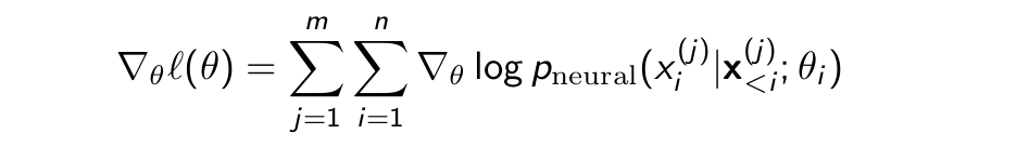
• Initialize θ0 = (θ1 , · · · , θn ) at random
• Compute ∇θℓ(θ) (by back propagation)
• θt+1 = θt + αt∇θℓ(θ)

Non-convex optimization problem, but often works well in practice

MLE Learning: Stochastic Gradient Descent

What if m = |D| is huge?

We have to sum the gradients for m samples from the dataset where each sample’s probablity is represented by an autoregressive model of n variables. If m is huge let’s assume = 10^6 then there will be at least 10^6*n computations per iteration if we use the Gradient Descent algorithm. This is an expensive cost for optimizing our model.

Solution? Monte-Carlo to the rescue.

The definition for Monte-Carlo

Definition for ∇θℓ(θ)

What’s missing?

Assuming the outer sum is what we need for computing expectation on sampling x from D and the inner sum highlighted in green is the random variable on which the expectation is being calculated then we are missing the probablities assosciated with the random variable being sampled from D.

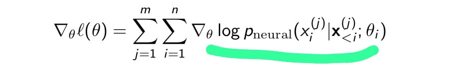
Adding m * 1/m (Assuming the sampling process is uniform)

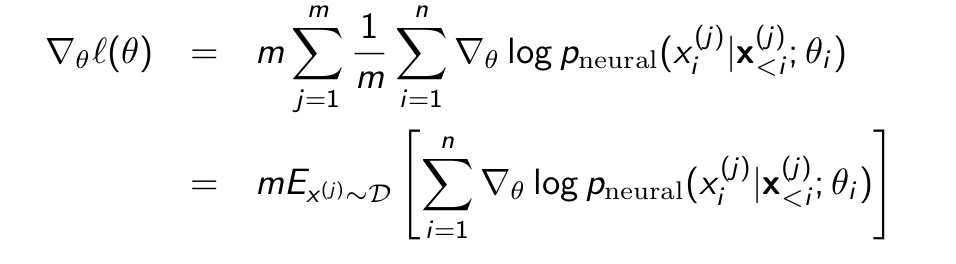
Then 1/m is the probablity associated for sampling each variable from D.

And by using the Monte-Carlo Estimation we can compute ∇θℓ(θ) in the following way.

Bias-Variance Trade Off

• If the hypothesis space is very limited, it might not be able to represent Pdata , even with unlimited data

  • This type of limitation is called bias, as the learning is limited on how close it can approximate the target distribution

• If we select a highly expressive hypothesis class, we might represent better the data

  • When we have small amount of data, multiple models can fit well, or even better than the true model. Moreover, small perturbations on D will result in very different estimates
  • This limitation is call the variance.

Sign-off

• For autoregressive models, it is easy to compute pθ (x)
• Natural to train them via maximum likelihood
• Higher log-likelihood doesn’t necessarily mean better looking samples
• Other ways of measuring similarity are possible (Generative Adversarial Networks, GANs)