About Link to heading

These blogs are my notes that represent my interpretation of the CS236 course taught by Stefano.

Recap: Learning a generative model Link to heading

Recall that we want to learn a probability distribution p(x) over images x such that sampling from this distribution gives us new images. In the last part we dived deeper into probability distributions. Finally we saw ways to learn a probability distrubution for a discriminative model using techniques like logistic regression or neural models.

Following that we will now understand how we can learn a probability distribution p(x) over images x using an autoregressive approach.

Autoregressive models Link to heading

The terminology of why an autoregressive model is called autoregressive is that it uses the information of previous states to predict the next state. Let’s understand this with an example

Assume that we have a 28x28 image with 784 pixels == 784 random variables.

In this image we assume an ordering of these variables a raster-scan ordering where we start from the top-left of the image and end at the bottom-right.

Using the logic mentioned in previous blog, we represent the distribution in the following way.

Assume
p(x1 , · · · , x784 ) = pCPT (x1 ; α1 ) plogit (x2 | x1 ; α2 ) plogit (x3 | x1 , x2 ; α3 ) · · · plogit (xn | x1 , · · · , xn−1 ; αn )
CPT = Conditional Probablity Table
logit = logistic model to represent p(x|y)

To Elaborate
pCPT (X1 = 1; α¹ ) = α¹ , p(X1 = 0) = 1 − α¹
plogit (X2 = 1 | x1 ; α² ) = σ(α0² + α1²x1)
plogit (X3 = 1 | x1 , x2 ; α³ ) = σ(α0³ + α1³x1 + α2³x2) (Note that αⁿ is not a power but a way to depict variables distinctly)

In this example we are making a modelling assumption where we are depicting our probablities in the form of parameterized functions. Also if we observe each pixel is dependent on all the pixels before it (following a raster-scan) which makes it an autoregressive model.

Autoregressive models: Architectures Link to heading

FVSBN Link to heading

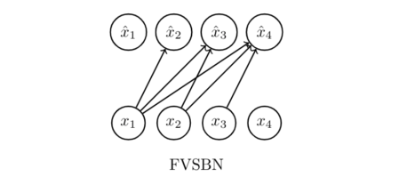
Given that the conditional variables Xi | X1 , · · · , Xi−1 are Bernoulli with parameters \

x̂i = p(Xi = 1|x1 , · · · , xi−1 ; αⁱ ) = p(Xi = 1|x<i ; αⁱ ) = σ(αⁱ0 + sum(αⁱjxj) for j = 1 to i-1)

How to evaluate? Link to heading

How do we evaluate p(x) = p(x1 , · · · , x784)?

An example: p(X1 = 0, X2 = 1, X3 = 1, X4 = 0)

From the previous equation.

p(X1 = 0) = 1 - x̂1 p(X2=1|X1=0) = x̂2 p(X3=1|X1=0, X2=1) = x̂3 p(X4=0|X1=0, X2=1, X3=1) = 1 - x̂4

Multiplying the conditionals gives us p(X1 = 0, X2 = 1, X3 = 1, X4 = 0) = (1 − x̂1) × x̂2 × x̂3 × (1 − x̂4)

How to sample? Link to heading

How to sample from p(x1 , · · · , x784 )?

• For x1_bar ∼ p(x1) (np.random.choice([1,0],p=[x̂1 , 1 − x̂1 ])) // making random choice of 1 and 0 based on probablity x̂1
• For sampling second pixel ~ p(x2) use p(x2 | x1 = x1_bar )
• For sampling third pixel ∼ p(x3 | x1 = x1_bar , x2 = x2_bar )
• and so on..

How many parameters (in the αⁱ vectors)? 1 + 2 + 3 + · · · + n ≈ n2 /2 Link to heading

Example Link to heading

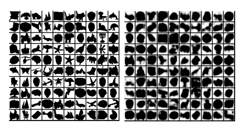Training data on the left (Caltech 101 Silhouettes). Samples from the model on the right.
Figure from Learning Deep Sigmoid Belief Networks with Data Augmentation, 2015.

NADE: Neural Autoregressive Density Estimation Link to heading

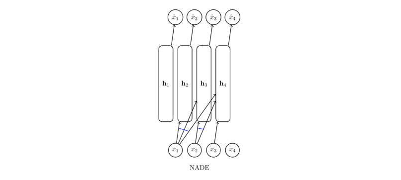
Idea: Instead of using logistic regression use a layer of neural network followed by logistic regression to represent probablity. Advantage is that it introduces non-linearity.

Example computation

We have to use a seperate matrix for each computation that increases the parameters and the time.

Instead share the parameters in a single matrix.

Example

Parameters Link to heading

If hi ∈ Rᵈ , how many total parameters? Linear in n: weights W ∈ Rᵈ*ⁿ ,
biases c ∈ Rᵈ , and n logistic regression coefficient vectors αi , bi ∈ Rᵈ⁺¹ .
Probability is evaluated in O(nd).

Samples Link to heading

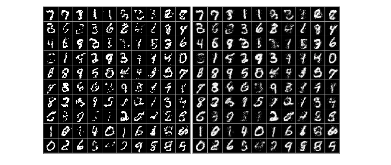
Samples from a model trained on MNIST on the left. Conditional probabilities x̂i on the right.

Figure from The Neural Autoregressive Distribution Estimator, 2011.

Modelling non-binary discrete random variables Link to heading

Till now we saw model architecures that help us model distributions having binary values. But what if we want to model non-binary random variables like an image having pixel values from 0 to 255.

To evaluate p(xi |x1 , · · · , xi−1 ). Instead of logistic function use a softmax function that generalizes the logistic by transforming a vector of K numbers into a vector of K probabilities that sum to 1.

Updated logic
x̂i = (pi¹ , · · · , piᵏ) = softmax(Aihi + bi)

where softmax is as follows

Modelling continuous distributions Link to heading

How to model continuous random variables Xi ∈ R? E.g., speech signals
Solution: let x̂ i parameterize a continuous distribution
E.g., uniform mixture of K Gaussians

RNADE Link to heading

Our goal is to model a continuous distribution.

Example: Assume that we want to learn a distribution p(xi |x1 , · · · , xi−1 )

Consider that x1,…,xi-1 are Gaussian distributions. Then xi can be represented as a mixture of Gaussians as shown below

The parameters of xi? mean and variance of the K Gaussian models.

Can use exponential exp(·) to ensure non-negativity

Are autoregressive models similar to autoencoders? Link to heading

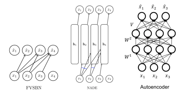
On the surface, FVSBN and NADE look similar to an autoencoder:
an encoder e(·). E.g., e(x) = σ(W² (W¹ x + b¹) + b²)
a decoder such that d(e(x)) ≈ x. E.g., d(h) = σ(Vh + c)

Here’s what the computation of NADE looks like

If we observe then the first equation seems to match with the definition of e(x) as NADE uses neural network to represent x in a compact way and then uses d(e(x)) to approximate a probability distribution from which we would sample the original data point xi.

But while an autoregressive model may seem like an autoencoder but the vice-versa is not true. Vanilla autoencoders do not learn any probablity distribution that we can sample from. Nor do they assume any ordering.

But an autoregressive model lets us parellelize operations. If we recall the NADE computation process. Then each hidden state is computed sequentially and not simultaneously. Whereas with an autoencoder we can get these hidden states in a single pass.

How? Let’s see that next..

MADE: Masked Autoencoder for Distribution Estimation Link to heading

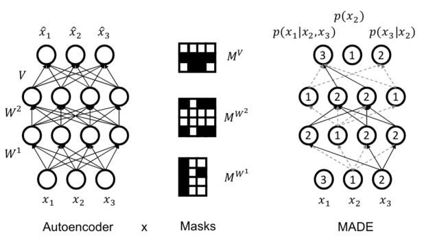
Challenge: An autoencoder that is autoregressive (DAG structure)

Solution: use masks to disallow certain paths (Germain et al., 2015). Suppose ordering is x2 , x3 , x1 , so p(x1 , x2 , x3 ) = p(x2 )p(x3 | x2 )p(x1 | x2 , x3 ).

• The unit producing the parameters for x̂2 = p(x2 ) is not allowed to depend on any input. Unit for p(x3 |x2 ) only on x2 . And so on… For each unit in a hidden layer, pick a random integer i in [1, n − 1].
• That unit is allowed to depend only on the first i inputs (according to the chosen ordering).
• Add mask to preserve this invariant: connect to all units in previous layer with smaller or equal assigned number (strictly < in final layer)

Some more model architectures that are modified to be autoregressive. Link to heading

Pixel RNN (Oord et al., 2016) Link to heading

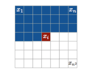
Model images pixel by pixel using raster scan order Each pixel conditional p(x_t | x₁:_t−1 ) needs to specify 3 colors p(x_t | x_1:t−1 ) = p(x_tred | x_1:t−1 )p(x_t green | x_1:t−1 , x_tred )p(x_tblue | x_1:t−1 , x_tred , x_tgreen ) and each conditional is a categorical random variable with 256 possible values. Conditionals modeled using RNN variants. LSTMs + masking (like MADE)

PixelCNN (Oord et al., 2016) Link to heading

Idea: Use convolutional architecture to predict next pixel given context (a neighborhood of pixels).
Challenge: Has to be autoregressive. Masked convolutions preserve raster scan order. Additional masking for colors order.

Summary of autoregressive models Link to heading

• Easy to sample from
  • Sample x0 ∼ p(x0 )
  • Sample x1 ∼ p(x1 | x0 = x 0 )
  • ···
• Easy to compute probability p(x = x)
  • Compute p(x0 = x0 )
  • Compute p(x1 = x1 | x0 = x0 )
  • Multiply together (sum their logarithms)
  • ···
  • Ideally, can compute all these terms in parallel for fast training
• Easy to extend to continuous variables. For example, can choose Gaussian conditionals p(xt | x<t ) = N (µθ (x<t ), Σθ (x<t )) or mixture of logistics
• No natural way to get features, cluster points, do unsupervised learning
• Next: learning