About
These blogs are my notes that represent my interpretation of the CS236 course taught by Stefano.
Part 2
Learning a generative model
In the last part we defined a statistical generative model represented as p(x) that lets us sample from this distribution to generate new images. But p(x) is unknown.
How do we learn it?
Before I go into it, we would be going into a lot of probablity terminologies that we will see. So whoever is reading I hope you are good with your probability. If not, there are a lot of videos to understand these terms in an awesome way. I will try my best though and hope it is understandable
Alright let’s get started then.
Probablity Distributions
Our goal is to learn a distribution that approximates the data that we are trying to generate. But what is a distribution? Let’s understand with an example.
Take an unbiased coin and toss it. What is the output? Write the probablity associated with it. Now write the probablity associated with the event that did not occur
It should look something like P(X = YourOutput) = 1/2 P(X != YourOutput) = 1 - 1/2
Well now you basically have the recipe to create a distribution.
Here is the checklist.
- A set of random variables
- The probablity associated with random distribution
Once you satisfy the checklist you plot the probablities associated with the random variable. Congratulations on creating a distribution for the first time or not..
Types
Discrete Probability Distributions
Probability distributions associated with random variables that are discrete in nature.
Examples(taken from the slides)
Bernoulli distribution: (biased) coin flip
D = {Heads, Tails}
Specify P(X = Heads) = p. Then P(X = Tails) = 1 − p.
Write: X ∼ Ber (p)
Sampling: flip a (biased) coin \
Categorical distribution: (biased) m-sided dice
D = {1, · · · , m}
P
Specify P(Y = i) = pi , such that
pi = 1
Write: Y ∼ Cat(p1 , · · · , pm )
Sampling: roll a (biased) die
Continuous Probablity Distribution
A continuous probability distribution is one in which a continuous random variable X can take on any value within a given range of values ‒ which can be infinite, and therefore uncountable. For example, time is infinite because you could count from 0 to a billion seconds, a trillion seconds, and so on, forever. Source(https://www.knime.com/blog/learn-continuous-probability-distribution)
Normally these distributions are defined using a probablity density function or PDFs not the file format:p
Example
Uniform Distribution
A Uniform distribution and is related to the events which are equally likely to occur. It is defined by two parameters, x and y, where x = minimum value and y = maximum value. It is generally denoted by u(x, y).
It is denoted as f(b)=1/y-x
Joint Probablity Distribution
The next topic is joint distribution which can be thought of as a distribution consisting of two or more random variables.
Examples
Flip of coins
Consider the flip of two fair coins; let A and B be discrete random variables associated with the outcomes of the first and second coin flips respectively. Each coin flip is a Bernoulli trial and has a Bernoulli distribution. If a coin displays “heads” then the associated random variable takes the value 1, and it takes the value 0 otherwise. The probability of each of these outcomes is 1/2.
To model the joint distribution we have to consider the all the possible cases.
In this case it will be
- P(A = Heads, B = Heads)
- P(A = Heads, B = tails)
- P(A = Tails, B = Heads)
- P(A = Tails, B = Tails)
Since the coins are fair the second coin won’t have any dependence on the first coin. In that case we can denote P(A, B) as the product of it’s probaility distribution
So each of the four cases are equally likely with a probablity of 1/4
and this joint distribution will be represented as P(A, B) = P(A)P(B) A,B -> {Heads, Tails}
P(A) = 1/2 A -> {Heads, Tails}
P(B) = 1/2 B -> {Heads, Tails}
Sampling from a distribution
Modelling a pixel’s color
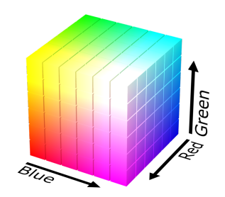
Let’s say we want to generate an image pixel by pixel in the RGB space.
For each channel assign a random variable. In this case -> 3 random variables
Red Channel R. Val(R) = {0, · · · , 255}
Green Channel G . Val(G) = {0, · · · , 255}
Blue Channel B. Val(B) = {0, · · · , 255}
The joint distribution p(r, g, b) can be used to sample pixels.
But how many parameters would be required to represent all the possibilities in this distribution
Considering that each channel has 256 possible values. It will mean 256^3 possibilites and assuming that we assign the last probablity as 1 - the sum of possible probablities
Then we get the number of parameters as 256^3 - 1
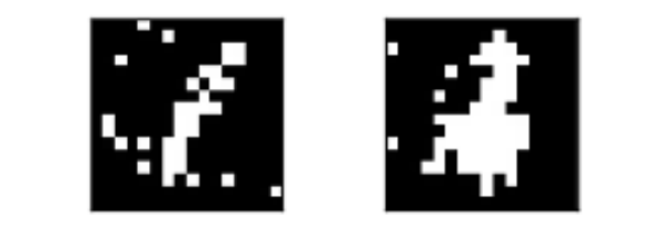
Modelling a binary image

Suppose X1 , . . . , Xn are binary (Bernoulli) random variables, i.e., Val(Xi ) = {0, 1} = {Black, White}.
Possible States? Each variable takes two values 0 and 1 for n variable - 2^n combinations/states
Sampling from p(x1 , . . . , xn ) generates an image
No of parameters required to represent the distribution = 2^n-1
Approximating distributions
Structure through Independence
From previous examples we see that sampling an image can be expensive. Can we make some assumptions??
Taking the binary image example what if we assume that the pixels of the binary image are independent.
In that case, p(x1 , . . . , xn ) = p(x1 )p(x2 ) · · · p(xn)
Possible states = Still 2^n
But parameters to represent this? Assuming each bernoulli distribution can be represented by a single parameter px where px is probablity of a pixel being 1 and 1-px the opposite
In that case we can represent 2^n states by just using n random variables
(Side note: In the previous case that won’t be possible as we don’t have independence between variables and so the conditional probability would need to be represented by some parameter and hence it was 2^n-1)
Cons?
Independence assumption is too strong. Model not likely to be useful
For example, each pixel chosen independently when we sample from it.
Structure through conditional independence
Using Chain Rule p(x1 , . . . , xn ) = p(x1 )p(x2 | x1 )p(x3 | x1 , x2 ) · · · p(xn | x1 , · · · , xn−1 )
How many parameters? 1 + 2 + · · · + 2n−1 = 2n − 1
p(x1 ) requires 1 parameter
p(x2 | x1 = 0) requires 1 parameter, p(x2 | x1 = 1) requires 1 parameter
Total 2^n parameters.
2^n − 1 is still exponential, chain rule does not buy us anything.
Now suppose Xi+1 ⊥ X1 , . . . , Xi−1 | Xi
What this means is that the variable Xi+1 is independent of variables from X1 to Xi-1 given Xi. In that case we can modify the p(x1,….,xn) as
p(x1 , . . . , xn ) = p(x1 )p(x2 | x1 )p(x3 | x2 ) · · · p(xn | xn−1 )
This forms the idea for Bayes Networks.
Bayes Network: General Idea
Use conditional parameterization (instead of joint parameterization)
For each random variable Xi , specify p(xi |xAi ) for set XAi of random variables
Then get joint parametrization as p(x1 , . . . , xn ) = mult( p(xi |xAi ) ) for i = 1 to n
Need to guarantee it is a legal probability distribution. It has to correspond to a chain rule factorization, with factors simplified due to assumed conditional independencies
Bayes Networks (Representation)
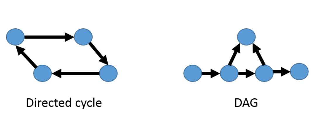 A Bayesian network is specified by a directed acyclic graph (DAG)
G = (V , E ) with:
A Bayesian network is specified by a directed acyclic graph (DAG)
G = (V , E ) with:
- One node i ∈ V for each random variable Xi
- One conditional probability distribution (CPD) per node, p(xi | xPa(i) ), specifying the variable’s probability conditioned on its parents’ values Graph G = (V , E ) is called the structure of the Bayesian Network
Defines a joint distribution: p(x1 , . . . xn ) = mult(p(xi | xPa(i) )) i∈V
Claim: p(x1 , . . . xn ) is a valid probability distribution because of ordering implied by DAG
Economical representation: exponential in |Pa(i)|, not |V |
Examples
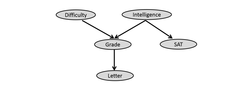
Consider the Bayes Network given.
How do we represent this network in terms of probablity?
For each node in the graph, consider the incoming edges those are the variables that the node depends on which also denotes the conditional independence on other variables given this incoming edges.
So,
p(difficulty) = p(difficulty)
p(intelligence) = p(intelligence)
p(grade) = p(grade | difficulty, intelligence)
p(letter) = p(letter | grade)
p(sat) = p(sat | intelligence)
The joint distribution corresponding to the above BN factors as
p(d, i, g , s, l) = p(d)p(i)p(g | i, d)p(s | i)p(l | g )
However, by the chain rule, any distribution can be written as
p(d, i, g , s, l) = p(d)p(i | d)p(g | i, d)p(s | i, d, g )p(l | g , d, i, s)
As represented by the Bayesian network. We are assuming the conditional independence.
D ⊥ I,
S ⊥ {D, G } | I ,
L ⊥ {I , D, S} | G .
Spam Classification
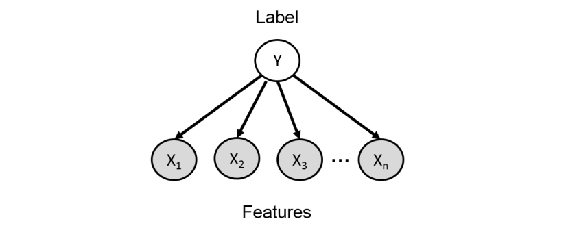 Classify e-mails as spam (Y = 1) or not spam (Y = 0)
- Let 1 : n index the words in our vocabulary (e.g., English)
- Xi = 1 if word i appears in an e-mail, and 0 otherwise
- E-mails are drawn according to some distribution p(Y , X1 , . . . , Xn )
Words are conditionally independent given Y
p(y , x1 , . . . xn ) = p(y) mult(p(xi | y )) for xi = 1 to n
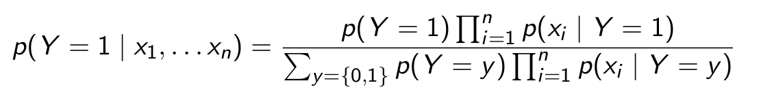
To evaluate p(y=1 | x1,…. xn) use Bayes Rule
Are the independence assumptions made here reasonable?
Philosophy: Nearly all probabilistic models are “wrong”, but many are
nonetheless useful
Discriminative versus generative models
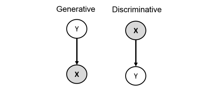
- Using chain rule p(Y , X) = p(X | Y )p(Y ) = p(Y | X)p(X). Corresponding Bayesian networks
- However, suppose all we need for prediction is p(Y | X). In the left model, we need to specify/learn both p(Y ) and p(X | Y ), then compute p(Y | X) via Bayes rule
- In the right model, it suffices to estimate just the conditional distribution p(Y | X)
- We never need to model/learn/use p(X)!
- Called a discriminative model because it is only useful for discriminating Y ’s label when given X
Example
Logistic Regression
For the discriminative model, assume that p(Y = 1 | x; α) = f (x, α).
Not represented as a table anymore. It is a parameterized function of x (regression)
- Has to be between 0 and 1
- Depend in some simple but reasonable way on x1 , · · · , xn
- Completely specified by a vector α of n + 1 parameters (compact representation)
Linear dependence: let z(α, x) = α0 + sum(αi*xi) for i = 1 to n .Then, p(Y = 1 | x; α) = σ(z(α, x)), where σ(z) = 1/(1 + e^−z ) is called the logistic function
Neural Models
In discriminative models, we assume that
p(Y = 1 | x; α) = f (x, α)
In previous example we have linear dependence
let z(α, x) = α0 + sum(αi*xi) for i = 1 to n
p(Y = 1 | x; α) = σ(z(α, x)), where σ(z) = 1/(1 + e −z ) is the logistic function
Dependence might be too simple
Solution?
Non-linear dependence: let h(A, b, x) = f (Ax + b) be a non-linear transformation of the inputs (features).
pNeural (Y = 1 | x; α, A, b) = σ(α0 + sum(αi*hi) for i = 1 to n)
- More flexible
- More parameters: A, b, α
Bayes Networks with Continuous Variables
Bayes Networks can also be used in case of continuous Variables. Here is an example
Mixture of 2 Gaussians
Consider that we want to map a bernoulli distribution Z to a gaussian distribution X.
Need to find p(x|z)
Z ∼ Bernoulli(p)
p(x|z) = p(X | (Z = 0)) ∼ N (µ0 , σ0 ) , p(X | (Z = 1)) ∼ N (µ1 , σ1 )
The parameters are p, µ0 , σ0 , µ1 , σ1
By mixing 2 Gaussians we have applied the concept of Bayes Networks where X depends on the variable Z.
Wrapping up
So this part we kind of got a lot into understanding about various probability distributions. How to sample from distributions, how to approximate them etc. Next part will pretty much focus on the same terminology but using a different class of models termed as autoregressive models. Until then bye!!